Course Notes
You can detail what you learned in the session within these pages. You can also use the Rmd markdown language and insert code chunks with CMD/CTRL + SHIFT + I.
Session 1
Session 2
Session 3
Session 4
Following session three, I spent time writing out the steps I might need to create one “Tidy” data frame that includes survey responses from each course. That looked like this:
Pseudocode into Code
- Read in various .csv files (all placed in common data folder)
- Remove metadata headers…first two columns (repeat for each file)
- Combine into one data frame
- Isolate Likert-type items
- Tidy data - gather into a longer table such that each response is its own entry
I then worked to write simplistic code to accomplish this task, which looked something like this:
read_csv(“data/file_name1.csv”)
file_name1_no_hd <- file_name1[-c(1,2), ]
all_data <- rbind(file_name1_no_hd, file_name2_no_hd,…)
all_likert <- all_data[ , -c(1:8, 10:17, 22, 29:38, 47, 49, 51, 53, 55, 57, 59, 61, 64:86)]
all_likert <- gather(all_likert, key = “Question”, value = “Response”, -ResponseId)
I then worked to identify strategies to streamline this process. For the next session, I am hoping to make progress on writing 1 or more functions to expedite the data import process. Additionally, I am hoping to begin some preliminary visualization work.
Session 5
Pulling data directly from Qualtrics (qualtRics package from rOpenSci) into project. Store private tokens in .Rprofile [usethis()]
Packages: usethis(); qualtRics(); gutenbergr()
Session 6
The Chronicle of Higher Education just released a special report, The Digital Campus: Big Data.
One of the articles touches on some interesting thoughtsaround data analytics and its relevance to the classroom, Can Data Make You a Better Teacher?. Moreover, it references a number of projects supported by Indiana University’s Center for Learning Analytics and Student Success, which is hosting its 2nd Annual Learning Analytics Summit this April.
More efficient ways to grab likert-type items from survey:
##demo_likert <- demo_survey %>%
  ##select_if(is.integer) %>%
  ##glimpse
Session 7
Thoughts/Notes
Collecting data & looking for relationships…then developing a hypothesis out of this exploration to collect new data and test for generalizability.
Analysis: an inference example
devtools::install_github("WFU-TLC/analyzr")## Skipping install of 'analyzr' from a github remote, the SHA1 (47c89d7a) has not changed since last install.
## Use `force = TRUE` to force installationlibrary(tidyverse)## ── Attaching packages ────────────────────────────────────────────────────────────────── tidyverse 1.2.1 ──## ✔ ggplot2 3.1.0 ✔ purrr 0.3.0
## ✔ tibble 2.0.1 ✔ dplyr 0.8.0.1
## ✔ tidyr 0.8.2 ✔ stringr 1.4.0
## ✔ readr 1.3.1 ✔ forcats 0.4.0## Warning: package 'tibble' was built under R version 3.5.2## Warning: package 'purrr' was built under R version 3.5.2## Warning: package 'dplyr' was built under R version 3.5.2## Warning: package 'stringr' was built under R version 3.5.2## Warning: package 'forcats' was built under R version 3.5.2## ── Conflicts ───────────────────────────────────────────────────────────────────── tidyverse_conflicts() ──
## ✖ dplyr::filter() masks stats::filter()
## ✖ dplyr::lag() masks stats::lag()library(analyzr)##
## Attaching package: 'analyzr'## The following object is masked _by_ '.GlobalEnv':
##
## sbcglimpse(sbc)## Observations: 362,592
## Variables: 8
## $ id <dbl> 1, 1, 1, 1, 1, 1, 1, 1, 1, 1, 1, 1, 1, 1, 1, 1, …
## $ name <chr> "lenore", "lenore", "lenore", "lenore", "lenore"…
## $ gender <chr> "female", "female", "female", "female", "female"…
## $ age <dbl> 30, 30, 30, 30, 30, 30, 30, 30, 30, 30, 30, 30, …
## $ years_edu <dbl> 16, 16, 16, 16, 16, 16, 16, 16, 16, 16, 16, 16, …
## $ utterance_clean <chr> "so you don't need to go borrow equipment from a…
## $ filler_type <chr> "um", "um", "um", "um", "um", "um", "um", "um", …
## $ filler_count <int> 0, 0, 0, 0, 0, 0, 0, 0, 0, 0, 0, 0, 0, 0, 0, 0, …head(sbc)To find out more about the data we can look at the data dictionary provided in the analyzr package with ?sbc.
sbc <- sbc %>% select(id, name, gender, age, years_edu, utterance_clean)
sbc <- sbc[complete.cases(sbc), ]
complete.cases identifies missing data cases (TRUE/FALSE). Subsets and only sends over complete cases. Other ways one might go about doing this. Publication might want to know what percent of data includes complete cases.
Tidy technique: use Filter(complete cases ###Extract dependent variable
sbc <-
  sbc %>%
  mutate(um = str_count(utterance_clean, "\\b(um|u=m)\\b")) %>%
  mutate(uh = str_count(utterance_clean, "\\b(uh|u=h)\\b"))

sbc
“\b(um|u=m)\b” -> \b indicates word boundary
  sbc <- gather(sbc, filler_type, filler_count, um:uh)

sbc
Question Why did I encounter an error here. When piping gather into sbc, funcitons below did not work as expected. Instead, I gathered into a new dataframe (sbc_2), then updated subsequent code chunks to account for this.
Analysis
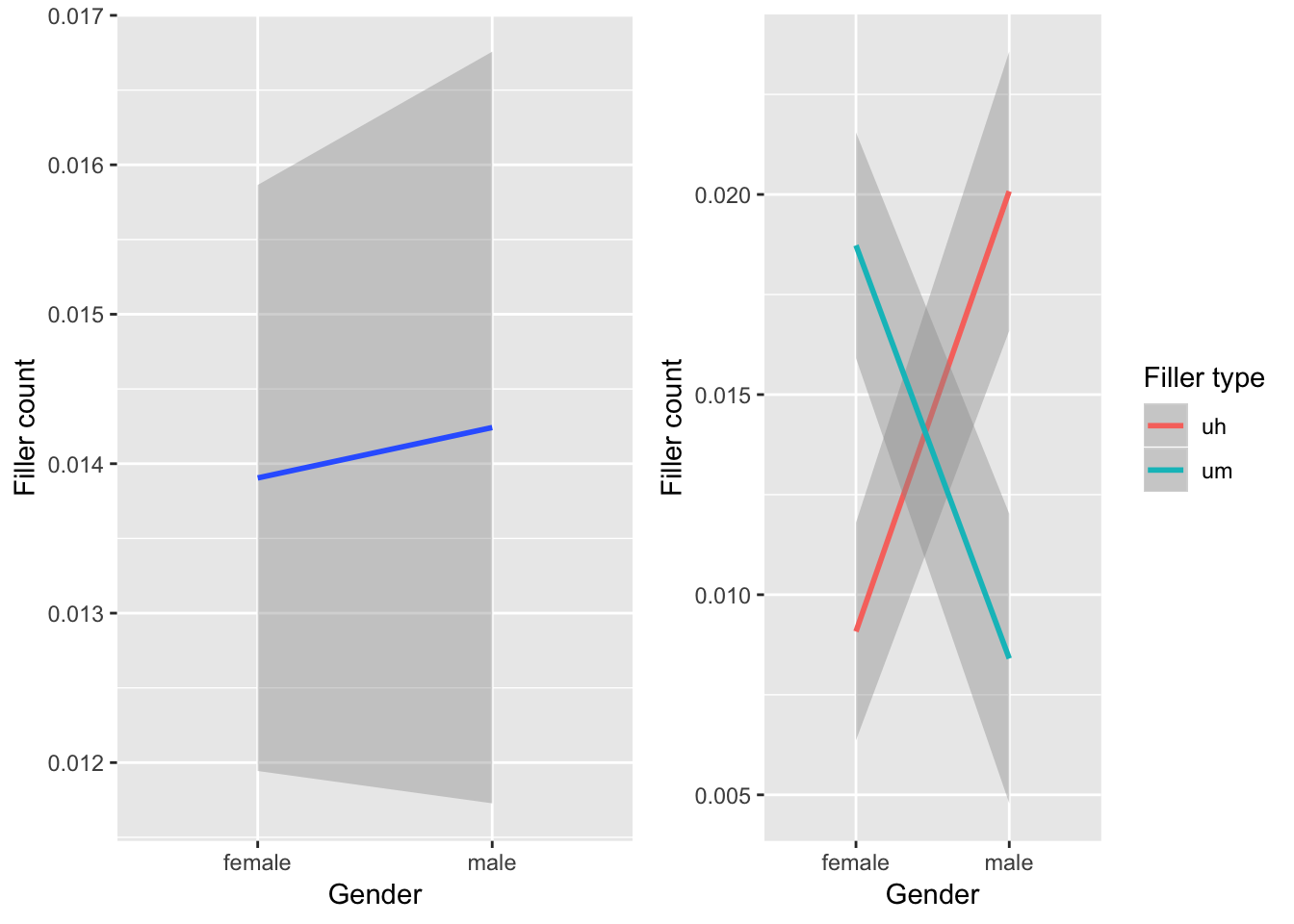
Gender
library(gridExtra)##
## Attaching package: 'gridExtra'## The following object is masked from 'package:dplyr':
##
## combinep1g <-
sbc %>%
ggplot(aes(x = gender, y = filler_count, group = 1)) +
geom_smooth(method = "lm") +
labs(x = "Gender", y = "Filler count")
p2g <-
sbc %>%
ggplot(aes(x = gender, y = filler_count, group = filler_type, color = filler_type)) +
geom_smooth(method = "lm") +
labs(x = "Gender", y = "Filler count", color = "Filler type")
gridExtra::grid.arrange(p1, p2, ncol = 2)
summary(glm(filler_count ~ gender, data = sbc_2, family = "poisson"))##
## Call:
## glm(formula = filler_count ~ gender, family = "poisson", data = sbc_2)
##
## Deviance Residuals:
## Min 1Q Median 3Q Max
## -0.1688 -0.1688 -0.1668 -0.1668 3.9878
##
## Coefficients:
## Estimate Std. Error z value Pr(>|z|)
## (Intercept) -4.27553 0.07142 -59.861 <2e-16 ***
## gendermale 0.02400 0.11531 0.208 0.835
## ---
## Signif. codes: 0 '***' 0.001 '**' 0.01 '*' 0.05 '.' 0.1 ' ' 1
##
## (Dispersion parameter for poisson family taken to be 1)
##
## Null deviance: 2721.7 on 22661 degrees of freedom
## Residual deviance: 2721.7 on 22660 degrees of freedom
## AIC: 3357.5
##
## Number of Fisher Scoring iterations: 6summary(glm(filler_count ~ gender * filler_type, data = sbc_2, family = "poisson"))##
## Call:
## glm(formula = filler_count ~ gender * filler_type, family = "poisson",
## data = sbc_2)
##
## Deviance Residuals:
## Min 1Q Median 3Q Max
## -0.2004 -0.1935 -0.1348 -0.1348 4.1949
##
## Coefficients:
## Estimate Std. Error z value Pr(>|z|)
## (Intercept) -4.7016 0.1250 -37.613 < 2e-16 ***
## gendermale 0.7936 0.1651 4.807 1.53e-06 ***
## filler_typeum 0.7239 0.1523 4.753 2.01e-06 ***
## gendermale:filler_typeum -1.5947 0.2502 -6.374 1.85e-10 ***
## ---
## Signif. codes: 0 '***' 0.001 '**' 0.01 '*' 0.05 '.' 0.1 ' ' 1
##
## (Dispersion parameter for poisson family taken to be 1)
##
## Null deviance: 2721.7 on 22661 degrees of freedom
## Residual deviance: 2676.5 on 22658 degrees of freedom
## AIC: 3316.3
##
## Number of Fisher Scoring iterations: 7gendermale is using female as reference level
Socioeconomic class
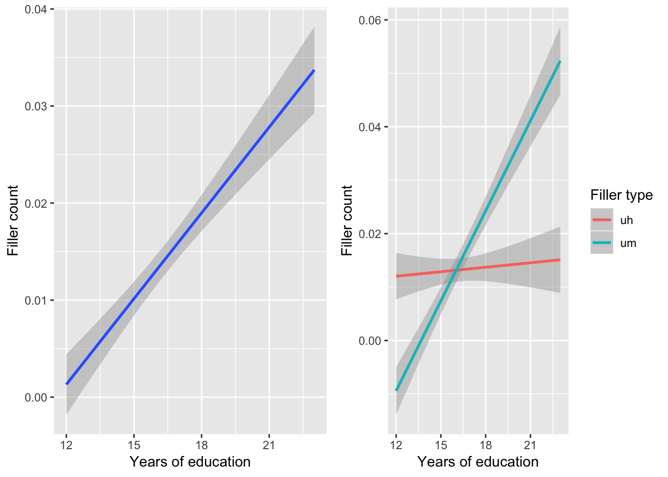
Using Education status as a proxy for socioeconomic class
p1ses <-
  sbc_2 %>%
  ggplot(aes(x = years_edu, y = filler_count, group = 1)) +
  geom_smooth(method = "glm") +
  labs(x = "Years of education", y = "Filler count")

# B
p2ses <-
  sbc_2 %>%
  ggplot(aes(x = years_edu, y = filler_count, color = filler_type, group = filler_type)) +
  geom_smooth(method = "glm") +
  labs(x = "Years of education", y = "Filler count", color = "Filler type")

gridExtra::grid.arrange(p1ses, p2ses, ncol = 2)
summary(glm(filler_count ~ years_edu, data = sbc_2, family = "poisson"))##
## Call:
## glm(formula = filler_count ~ years_edu, family = "poisson", data = sbc_2)
##
## Deviance Residuals:
## Min 1Q Median 3Q Max
## -0.2961 -0.1852 -0.1535 -0.1535 4.4219
##
## Coefficients:
## Estimate Std. Error z value Pr(>|z|)
## (Intercept) -7.44534 0.36186 -20.57 <2e-16 ***
## years_edu 0.18775 0.02032 9.24 <2e-16 ***
## ---
## Signif. codes: 0 '***' 0.001 '**' 0.01 '*' 0.05 '.' 0.1 ' ' 1
##
## (Dispersion parameter for poisson family taken to be 1)
##
## Null deviance: 2721.7 on 22661 degrees of freedom
## Residual deviance: 2642.6 on 22660 degrees of freedom
## AIC: 3278.5
##
## Number of Fisher Scoring iterations: 7Session 8
Pre-work
I will be attending the Learning Technology Consortium meeting at Duke this week. As part of this meeting (the group meets twice a year, rotating hosting duties among 10 institutions), representatives from each school provide updates on current work in learning technologies at their institution. WFU’s update has taken two forms:
- LTC Update Podcast: Provides an overview of a few things of note.
- Written update
While the report itself does not involve any data, I wanted to practice writing the update using the Tufte package in R, since this is one route I might go to represent recurring survey feedback reports for OLEC. The package allows for publishing .Rmd files as PDF or HTML files using the style of Edward Tufte’s written texts. Some central features of this style include: marginal notes and figures, in-line images & figures, and specific heading & font styles. I’ve been mostly successful in publishing it, but I believe I may be doing something wrong with my yaml file or the structure of my folder, since certain behaviors end up breaking my site in unexpected ways.
References
Copyright © 2018 Allen Brown. All rights reserved.